In my last post I made an argument that felt, to me, like stating the obvious — but one I couldn’t find anyone else putting into words: backtracking is just counting. If your search space is a product of small independent choices, a depth‑first walk through it is the same object as incrementing a mixed‑radix number — an odometer. And a “prune” is just you refusing to descend into a number you can already see is doomed. I wrote the full version of that up: backtracking as a bijection to the integers.
This is the second half of that thought. And I think it’s the half that finally explains why dynamic programming works — not what it is, but the reason it gets to be fast.
Three densities of one walk
Most of us were taught three “algorithms”: brute force, backtracking, and dynamic programming. I’ve come to think of them as three densities of the same walk through a state space, and I want to show you the exact place where the density changes.
Picture the odometer ticking in real time, one mixed‑radix number at a time. Now read the walk three ways:
- The dense walk (brute force). The counter ticks through every number. You visit all of them.
- The pruned walk (backtracking). The counter still ticks in order, but you skip any number that fails an admissibility test. You visit every viable number.
- The sparse walk (dynamic programming). Here’s the move. You still let the counter tick, but you stop and do work only when the state changes. A whole run of consecutive numbers that all describe the same situation gets fast‑forwarded over. You visit each distinct situation exactly once.
That last step is the entire content of dynamic programming. Everything else — the table, the memo map, the “find the recurrence” ritual — is just how you make that fast‑forward efficient instead of literal.
The projection is the whole problem
To say “the state changes” I need one precise idea, and it’s small enough to write on a whiteboard in one line. Call it κ: a function from an odometer position to a canonical state.
A state is any function of the search that is predictive of the future — i.e., two positions that κ maps to the same value are interchangeable.
That’s it. And “predictive of the future” is just the textbook’s optimal substructure, wearing a different shirt. The reason you’re allowed to collapse two different paths into one state is that, from that state onward, the path you took to get there is irrelevant — only the state matters. If that’s true for your problem, you have a DP. If it’s not, you don’t, and no amount of clever memoizing will save you.
So the speedup of a DP, in one ratio, is:
$$\frac{\text{positions the counter visits}}{\text{distinct states it visits}}$$
Backtracking visits viable positions; DP visits states. Same counter, same order, different stopping rule — and that gap is exactly the speedup.
The principle, stated once
Strip the examples away and the whole argument is five objects, one ordering, and one license.
The objects.
- The odometer. $n$ independent choices, choice $i$ drawn from a finite base $B_i$. A position is $\omega = (d_1,\dots,d_n)$; all positions form the mixed-radix space $\Omega = \prod_i B_i$, with $|\Omega| = \prod_i |B_i|$.
- The tick. A fixed total order on $\Omega$ — the lexicographic increment. A walk is a sequence of positions in that order.
- Admissibility. A prefix predicate $A$ — your
admissible. Pruning is refusing to descend into a position that fails $A$. - The projection. $\kappa : \Omega \to S$ — your
canonical— maps a position to its canonical state. The position may be a prefix of the plan — what the walk passes through — or the plan in full — where it lands; the ordering below holds at either level, since it holds for any function composed after any filter. - The reward. A local weight $r$ on the tick’s transitions, or a terminal $R$ — the thing you maximize, orthogonal to the projection.
The ordering. The two moves compose into one chain — three walks over one counter:
$$|\Omega| \xrightarrow{A} |\Omega_A| \xrightarrow{\kappa} |\kappa(\Omega_A)| \qquad\qquad \text{brute force}\rightarrow\text{backtracking}\rightarrow\text{DP}$$
Each arrow is one of the two things you can do to a search: $A$ throws out the doomed, $\kappa$ throws out the redundant — the left is pruning, the right is sparsification. Statically, the whole argument is one line:
$$|\kappa(\Omega_A)| \leq |\Omega_A| \leq |\Omega|$$
DP is no bigger than backtracking, which is no bigger than brute force. Each leg is $\leq$ for a boring, exact reason:
- $|\Omega_A| \leq |\Omega|$, because $A$ is a filter — $\Omega_A \subseteq \Omega$. Equality iff nothing gets pruned: backtracking collapses to brute force.
- $|\kappa(\Omega_A)| \leq |\Omega_A|$, because $\kappa$ is a function — a many‑to‑one map can’t produce more images than it has inputs. Equality iff $\kappa$ is injective on the admissible set: DP collapses to backtracking.
So the inequality itself is almost trivial. The teeth are in the strictness. The second leg is strict exactly when some state has two or more admissible preimages — that’s the moment a DP actually earns its keep, and the only number that matters.
And strictness needs a license. One condition — the lumping rule: $\kappa$ is a legal projection if and only if it respects the value‑to‑go:
$$\kappa(\omega) = \kappa(\omega’) \Longrightarrow V(\omega) = V(\omega’).$$
In words: two positions that κ merges must have the same future. That is just optimal substructure — the Markov property — stated as a congruence on the odometer. Include too little in $\kappa$ and you merge states that should differ — you get a wrong answer, the classic “forgot a dimension” bug. Include too much and you over-split, lose the speedup, and slide back toward backtracking.
And the two ends live independently: strictness is your speed — you visit fewer things; the lumping rule is your correctness — the things you merged were safe to merge. You can have a strict κ that’s wrong, or a safe κ that’s useless — injective, so you gained nothing. A dynamic program is the sweet spot where the second inequality is strict and the lumping rule holds — make $\kappa$ exactly the coordinates the future reads, no more, no less.
The recurrence, on states. On the state space $S$, with the successor relation induced by the tick and projected through $\kappa$:
$$\tilde V(s) = \max_{s ,\to, s’} \big( r(s,s’) + \tilde V(s’) \big),$$
evaluated in the tick’s order, deduplicated — that is, in a topological order of the state DAG. The max is the choice; evaluating each state exactly once is the sparsity. “Deduplicated, in topological order” is the whole second half of this post — here is that program.
The principle, as a program
Here it is, generic, with the three layers commented so you can see them for yourself:
// The sparse walk: let the odometer tick, but do work only on *new* states.
std::vector<int> omega(n, 0);              // the odometer (mixed-radix digits)
unordered_map<State, T> V;                 // the DP table, indexed by canonical state

auto tick = [&]{                            // increment the mixed-radix counter
    for (int i = n - 1; i >= 0; --i) {
        if (++omega[i] < base[i]) return true;   // carry handled naturally
        omega[i] = 0;
    }
    return false;                           // every digit exhausted
};

do {
    if (!admissible(omega)) continue;       // <-- LAYER 2: backtracking (prune)
    State s = canonical(omega);             // <-- the projection κ
    if (V.count(s)) continue;               // <-- LAYER 3: DP (skip seen states)
    V[s] = best_transition_from(s);         // do the work, exactly once per state
} while (tick());                           // <-- LAYER 1: the odometer itself
Read the three continues top to bottom and you’ve seen the whole argument: prune the doomed, project to a state, skip what you’ve already solved. The dense walk is the tick(). Backtracking is the first filter. DP is the second.
One honest caveat, because I won’t pretend otherwise: in practice you would never actually tick the counter and discard. That would be absurdly wasteful — you’d still touch every position. The efficient implementation fills the state table directly, in topological order. But the picture is identical: the table is the sparse walk, made concrete. The counter is a way of seeing the table, not of building it. (And one other small license the sketch takes: it tests admissible on the full position, where the backtracking of the last post tests it on partial positions and jumps whole doomed runs. The densities don’t change; only the size of the jump does.)
A worked example: House Robber
Take LeetCode 198. n houses with values v[i]; you may not rob two adjacent houses; maximize the sum.
The counter here is a binary string — for each house, rob (1) or skip (0). So the three densities, for n = 10:
| Walk | What it visits | Count |
|---|---|---|
| Dense (odometer) | every rob/skip string | 2¹⁰ = 1,024 |
| Pruned (backtracking) | strings with no two adjacent 1s (a Fibonacci count) | 144 |
| Sparse (DP) | distinct states | 20 |
That 1024 → 144 → 20 is the whole story, in one table — and it’s the strictness from the principle, made loud. The prune layer removes the “two adjacent robberies” strings, a Fibonacci’s worth of them: $F_{12} = 144$. And look at the two cuts: $1024 / 144 \approx 7.1$, and $144 / 20 = 7.2$ — two almost-equal 7× cuts. That balance is a happy accident of the magnitudes and it won’t always hold; what always holds is that each arrow is a real compression of the same walk, and the gap end to end — 1024 → 20 — is 51×.
One honest footnote on bookkeeping: the first two rows count plans — whole strings, the leaves of the walk — while the last row counts the situations the walk passes through. Every number is real, and each arrow is a real compression; only the grain differs. (Count the nodes a pruned DFS actually touches — every admissible prefix, not just its leaves — and the count is 375; the last cut is wider still.)
The sparse layer does the dramatic thing: it notices that the future depends on only two things — which house you’re at, and whether the previous one was robbed. In the notation of the principle, $\kappa$ maps each prefix of the string to how far in it is, and what the trailing digit is. Per house you carry two states, A(i) and B(i), and that’s the table:
A(i) = max(A(i-1), B(i-1))     // skip house i: the previous was either way
B(i) =      A(i-1) + v[i]      // rob house i: the previous MUST have been skipped
A and B are the two canonical states — (i, 0) and (i, 1). You’re carrying two numbers forward instead of walking a thousand‑node tree, and the reason you’re allowed to is that κ threw away everything the future doesn’t use. The odometer is still the thing generating the transitions; the DP is just the odometer’s shadow on the state wall.
Now change κ: a budget allocator
If the previous example made you think “fine, but that’s a neat trick for this problem,” here’s the generalization. Same machine, new projection.
You have three projects, three effort levels each (L ∈ {0,1,2}), a budget of 10, and you maximize value:
| L=0 | L=1 | L=2 | |
|---|---|---|---|
| P1 cost / value | 0 / 0 | 3 / 10 | 5 / 15 |
| P2 cost / value | 0 / 0 | 4 / 12 | 6 / 20 |
| P3 cost / value | 0 / 0 | 2 / 8 | 7 / 25 |
With cost limit $$B=10$$.
The counter is the triple (L1, L2, L3) — base 3, so 27 dense positions. Here’s a (deliberately non‑contiguous) slice of the walk, all three layers visible at once:
| Odometer | cost sum | pruned? | κ = spent |
|---|---|---|---|
| (0,1,1) | 6 | ✓ | 6 |
| (0,1,2) | 11 | ✗ | — |
| (0,2,0) | 6 | ✓ | 6 |
| (1,0,1) | 5 | ✓ | 5 |
| (1,1,2) | 14 | ✗ | — |
| (2,0,0) | 5 | ✓ | 5 |
See the bolded repeats? (0,1,1) and (0,2,0) are two different effort plans that land on the same spent budget; same with (1,0,1) and (2,0,0). That’s the lumping rule doing its work on the ground — different paths, same future, one state.
Across the whole space the three densities are 27 → 16 → 10: 27 plans, 16 that fit the budget, and the 16 landing on 10 states — and, as it happens, every budget value from 0 to 10 is reachable, so the 10 states are simply all the budgets. The best_value(stage, spent) table holds 3 live cells at stage one, 7 at stage two, and 10 in the final row — twenty reachable cells, coincidentally the same count as the robber’s table, for entirely different reasons. The optimum — 35, via plan (1,0,2) — is read off that final row of ten states, never by walking sixteen plans.
All three layers in one picture, then: the walk on the right, the states it projects onto on the left.
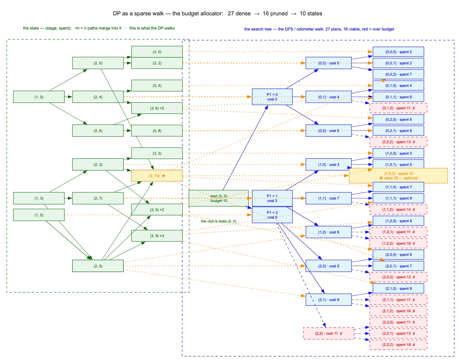
Look at the fibers, since that’s the point. Every orange line is a plan being forgotten: the tree remembers the route, the state doesn’t. And every state is exactly as tall as its thickest bundle of preimages — the places where two or three plans pile onto one (the ×2, the ×3) are the places where the walk is thickest, and the table is where it is thinnest. One walk, three grains, and the gap between them is something you can now count by eye.
In the math, with $c(i,L)$ and $v(i,L)$ read from the table above.
The κ (canonical state): a state, at stage $i$, is the stage and the spent-so-far — the running sum is the κ:
$$\kappa_i(L_1, \dots, L_i) = \left( i, \textstyle\sum_{j \le i} c(j, L_j) \right)$$
Notice what κ does not read: the value. Each option is a (cost, value) pair — the standard multiple‑choice shape — but the projection is a function of the running cost alone: the budget is the constraint, and the constraint is what the future depends on. The values are just the payload — the reward $r$ from the principle — maximized on top of the states. So the number of states — the sparsity — is driven purely by the cost structure, and κ can be designed before you look at a single value. The projection is about the dependencies, never the objective. (If you’d rather a single value per project, with effort level just scaling cost, that’s a fine variant too — but the per‑option version is the one that makes the many‑to‑one merges most visible, and the merges are the point.)
The recurrence, forward — in best_value(stage, spent) form:
$$BV(0,0) = 0, \qquad BV(0,s) = -\infty \ \text{ for } s > 0$$ $$BV(i, s) = \max_{\substack{L \in {0,1,2} \ s - c(i,L) \ge 0}} \Bigl[ BV(i-1, s - c(i,L)) + v(i, L) \Bigr]$$ $$\text{answer} = \max_{0 \le s \le B}, BV(n, s)$$
The same κ, read backwards — the form most of us first meet in the textbook, with remaining budget $b$:
$$ V(i,b) = \max_{\substack{L \in {0,1,2} \ c(i,L) \le b}} \Bigl[ v(i,L) + V(i+1, b - c(i,L)) \Bigr], \qquad V(n+1, b) = 0, \qquad \text{answer} = V(1, B) $$
Same shadow, cast from the other end of the walk: forward, the last decision materializes as a row of 10 cells; top‑down, it is the final max inside a row of 7. Either way it lands on 35, with the budget spent to exactly 10.
One honest word on scale: with three projects nothing here is a performance event — the full (stage, spent) grid is $4 \times 11 = 44$ cells, and the 27 plans fit in a pocket. This example is a mechanism demo, not a scale demo; the scale was the robber. Its job is to show that the machine survives a change of κ.
Same recurrence shape as the robber. Same tick, same lumping rule. Only κ changed. In the robber, κ is a trailing bit; here, a running sum. The machine is identical; the projection is the only thing that’s problem‑specific.
The one sentence
I keep coming back to a single line, and I think it’s the one worth leaving you with:
The recurrence is universal. κ is the content.
“Find the recurrence” is what we’re taught to do, and it’s the part everyone memorizes. But the thinking — the part that actually generalizes from problem to problem — is the smaller, quieter question: what does the future depend on? Answer that, and you have κ. Answer that, and the dense walk thins itself into a sparse one, and the table writes itself.
I’ll confess the honest version of why this matters to me personally. I’ve been seeing this shape for a long time — long before I had the words for it. I built project‑scheduling tools for years, and the instinct that kept showing up in them was density: I’d look at a plan and I didn’t want to know the list of tasks, I wanted to know where it was thick, where it would clog, where a single point of overload would take the whole portfolio down with it. That’s the same instinct as the one in this post, wearing a different jacket. A schedule that’s “full” but strategically chaotic is a dense walk; a plan that breathes is a sparse one. The odometer, the projection, the budget, the calendar — they’re all the same argument that the future is a low‑dimensional function of the present.
So: next time a problem resists, don’t ask “what’s the recurrence.” Ask “what’s κ?” Count the positions, count the states, and let the gap between the two numbers tell you whether you’re holding a dynamic program at all.